The method of Connor and Trinquart (Stat Med 2021) estimates the RMTL in the presence of competing risks. This function is a modification of their R code. Estimation functions are identical; input handling and output have been adapted.
estimate_rmtl(
  data,
  exposure = NULL,
  time,
  time2 = NULL,
  event,
  event_of_interest = 1,
  weight = NULL,
  tau = NULL,
  reach_tau = c("warn", "stop", "ignore"),
  conf.level = 0.95
)
Arguments
- data
Data frame (tibble).
- exposure
Optional. Name of exposure variable within the
data. If omitted, will return unstratified RMTL.- time
Name of time variable within the
data. By default, this is the event time. Iftime2is also given, this is the entry time, as perSurvstandard.- time2
Optional. Name of the variable within the
dataindicating the exit (event) time. If omitted,timeis the event time, as perSurvstandard.- event
Name of event variable within the
data. Can be integer, factor, character, or logical. The reference level indicates censoring and is taken as the first level of the factor, the lowest numeric value (usually0), orFALSEfor a logical variables. Other levels are events of different types. If no competing risks, the alternative level, e.g.1, indicates the event (e.g., death).- event_of_interest
Optional. Indicator for which of the non-censoring events is of main interest. Others are treated as competing. Defaults to
1, i.e., the first non-censoring event.- weight
Optional. Weights, such as inverse-probability weights or survey weights. The default (
NULL) uses equal weights for all observations.- tau
Optional. Time horizon to restrict event times. By default, the latest time in the group with the shortest follow-up. Prefer a user-defined, interpretable time horizon.
- reach_tau
Optional. How to handle provided
tauvalues that are not reached in one of the exposure categories."warn"Default. Display a warning and estimate RMTL and its difference in those exposure categories wheretauis reached."stop"Stop with an error iftaunot reached in one or more of the exposure categories."ignore"Ignore exposure categories wheretauis not reached; estimate RMTL and its difference in those exposure categories wheretauis reached.
If
tauis not reached in any of the exposure categories, the function always stops with an error.- conf.level
Optional. Confidence level. Defaults to
0.95.
Value
List:
tauTime horizon.rmtlTibble with absolute estimates of RMTL, per exposure group if given.rmtdiffTibble with contrasts of RMTL between exposure groups, compared to a common reference (the first level). Empty tibble if no exposure variable given.cifTibble with cumulative incidence function for the event of interest:exposureExposure group.timeEvent time.estimateAalen-Johansen estimate of cumulative incidence function withse,conf.low, andconf.high.
Details
Differences to the original function rmtl::rmtl():
Pass data as a data frame/tibble and select variables from it.
Allow for different variable types in the
eventvariable.Use
Survconventions for entry/exit times (time,time2).Allow for exposure groups where
tauis not reached.Return contrasts in restricted mean time lost as comparisons to the reference level instead of all pairwise comparisons.
Add origin (time 0, cumulative incidence 0) to the returned cumulative incidence function for proper plotting.
Return results as a list of tibbles. Do not print or plot.
References
Conner SC, Trinquart L. Estimation and modeling of the restricted mean time lost in the presence of competing risks. Stat Med 2021;40:2177–96. https://doi.org/10.1002/sim.8896.
Examples
data(cancer, package = "survival")
cancer <- cancer %>% dplyr::mutate(
status = status - 1, # make 0/1
sex = factor(sex, levels = 1:2, labels = c("Men", "Women")))
result <- estimate_rmtl(
data = cancer,
exposure = sex,
time = time,
event = status,
tau = 365.25) # time horizon: one year
result
#> $tau
#> [1] 365.25
#>
#> $rmtl
#> # A tibble: 2 × 5
#> exposure estimate se conf.low conf.high
#> <chr> <dbl> <dbl> <dbl> <dbl>
#> 1 Men 124. 10.4 103. 144.
#> 2 Women 67.7 10.8 46.5 88.8
#>
#> $rmtdiff
#> # A tibble: 2 × 6
#> exposure estimate se conf.low conf.high p.value
#> <chr> <dbl> <dbl> <dbl> <dbl> <dbl>
#> 1 Men 0 NA NA NA NA
#> 2 Women -56.0 15.0 -85.4 -26.7 0.000183
#>
#> $cif
#> # A tibble: 110 × 6
#> exposure time estimate se conf.low conf.high
#> <chr> <dbl> <dbl> <dbl> <dbl> <dbl>
#> 1 Men 0 0 NA NA NA
#> 2 Women 0 0 NA NA NA
#> 3 Men 11 0.0217 0.0124 -0.00259 0.0461
#> 4 Men 12 0.0290 0.0143 0.000995 0.0570
#> 5 Men 13 0.0435 0.0174 0.00945 0.0775
#> 6 Men 15 0.0507 0.0187 0.0141 0.0873
#> 7 Men 26 0.0580 0.0199 0.0190 0.0970
#> 8 Men 30 0.0652 0.0210 0.0240 0.106
#> 9 Men 31 0.0725 0.0221 0.0292 0.116
#> 10 Men 53 0.0870 0.0240 0.0399 0.134
#> # ℹ 100 more rows
#>
# Make simple plot
library(ggplot2)
library(dplyr)
#>
#> Attaching package: ‘dplyr’
#> The following objects are masked from ‘package:stats’:
#>
#> filter, lag
#> The following objects are masked from ‘package:base’:
#>
#> intersect, setdiff, setequal, union
library(tidyr)
result$cif %>%
ggplot(mapping = aes(x = time, y = estimate, color = exposure)) +
geom_step() +
scale_x_continuous(breaks = seq(from = 0, to = 365, by = 60)) +
labs(x = "Time since start of follow-up in days",
y = "Cumulative incidence")
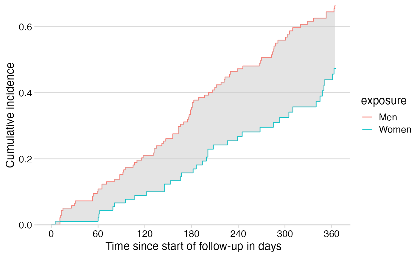
 # Make fancier plot with a shaded area for the RMTL difference
df_ribbon <- result$cif %>%
select(exposure, time, estimate) %>%
pivot_wider(names_from = exposure,
values_from = estimate,
names_repair = ~c("time", "surv", "surv2")) %>%
filter(time < 365.25) %>% # tau for RMST
arrange(time) %>% # carry forward survival values per stratum
fill(surv) %>%
fill(surv2)
result$cif %>%
ggplot() +
geom_step(mapping = aes(x = time, y = estimate, color = exposure)) +
scale_x_continuous(breaks = seq(from = 0, to = 365, by = 60)) +
scale_y_continuous(expand = expansion()) +
labs(x = "Time since start of follow-up in days",
y = "Cumulative incidence") +
cowplot::theme_minimal_hgrid() +
geom_stepribbon(data = df_ribbon,
mapping = aes(x = time, ymin = surv, ymax = surv2),
fill = "gray80", alpha = 0.5)
# Make fancier plot with a shaded area for the RMTL difference
df_ribbon <- result$cif %>%
select(exposure, time, estimate) %>%
pivot_wider(names_from = exposure,
values_from = estimate,
names_repair = ~c("time", "surv", "surv2")) %>%
filter(time < 365.25) %>% # tau for RMST
arrange(time) %>% # carry forward survival values per stratum
fill(surv) %>%
fill(surv2)
result$cif %>%
ggplot() +
geom_step(mapping = aes(x = time, y = estimate, color = exposure)) +
scale_x_continuous(breaks = seq(from = 0, to = 365, by = 60)) +
scale_y_continuous(expand = expansion()) +
labs(x = "Time since start of follow-up in days",
y = "Cumulative incidence") +
cowplot::theme_minimal_hgrid() +
geom_stepribbon(data = df_ribbon,
mapping = aes(x = time, ymin = surv, ymax = surv2),
fill = "gray80", alpha = 0.5)