Installation
The khsmisc package can be installed from GitHub:
# if "remotes" library is missing, install it first:
#   install.packages("remotes")
remotes::install_github("stopsack/khsmisc", build_vignettes = TRUE)
To access the documentation after installing the package, run
help("khsmisc")or
vignette("khsmisc")Setting up a new RMarkdown
After successfully installing khsmisc:
-
Create an RMarkdown file
RStudio: File > New File > R Markdown… > From Template > khsmisc RMarkdown template
Customize the YAML header
- Change the
title:andauthor:fields. - The date will automatically be updated when compiling the document.
- Note that this type of code, “YAML,” is sensitive to exact identation. Every indentation is done by exactly two spaces.
-
Load the package
The template provides code that will load a number of packages via the khsverse meta-package:
library(khsverse)- To just load the khsmisc package by itself, replace
library(khsverse)bylibrary(khsmisc). - The template also includes code to set graphics output to SVG format. If PNG output is preferred or the svglite package is not installed, that part can be deleted.
-
Knit the RMarkdown a first time
The RMarkdown is ready to be compiled using the Knit button. An HTML document should open that has nothing but a title and the startup messages of
khsverseabout all the packages it loads. If an an error message is shown instead, perhaps one of the packages was not installed properly?Learn more about the syntax of RMarkdown in the RStudio cheatsheets.
Data handling
Load the TCGA BLCA dataset
Participant and tumor data from the Cancer Genome Atlas Bladder
Cancer “cohort” (BLCA) will be used in their published 2017
version. Insert a new R chunk into the markdown (toolbar:
Insert > R), and add code for reading a
tab-separated file (“TSV”). The code retrieves the file
data_clinical_patient.txt, which can be downloaded as part
of the cBioPortal
TCGA-BLCA tarball (276 MB). A copy of just the “clinical” dataset is
available in the extdata directory of the khsmisc package.
The first four lines of the TSV file are skipped because they contain
meta-data.
clinical <- read_tsv(file = system.file("extdata", "data_clinical_patient.txt",
                                        package = "khsmisc", mustWork = TRUE),
                     skip = 4)
#> Rows: 411 Columns: 83
#> ── Column specification ────────────────────────────────────────────────────────
#> Delimiter: "\t"
#> chr (81): OTHER_PATIENT_ID, PATIENT_ID, FORM_COMPLETION_DATE, PROSPECTIVE_CO...
#> dbl  (2): AGE, DAYS_TO_INITIAL_PATHOLOGIC_DIAGNOSIS
#>
#> ℹ Use `spec()` to retrieve the full column specification for this data.
#> ℹ Specify the column types or set `show_col_types = FALSE` to quiet this message.
An inventory of the dataset:
varlist(clinical) %>%
  print(n = 15)  # show the first 15 lines of output
#> # A tibble: 83 × 4
#>    name                               n class     label
#>    <chr>                          <dbl> <chr>     <chr>
#>  1 OTHER_PATIENT_ID                 411 character NULL
#>  2 PATIENT_ID                       411 character NULL
#>  3 FORM_COMPLETION_DATE             411 character NULL
#>  4 PROSPECTIVE_COLLECTION           411 character NULL
#>  5 RETROSPECTIVE_COLLECTION         411 character NULL
#>  6 DAYS_TO_BIRTH                    411 character NULL
#>  7 SEX                              411 character NULL
#>  8 HEIGHT                           411 character NULL
#>  9 WEIGHT                           411 character NULL
#> 10 RACE                             411 character NULL
#> 11 ETHNICITY                        411 character NULL
#> 12 HISTORY_OTHER_MALIGNANCY         411 character NULL
#> 13 HISTORY_NEOADJUVANT_TRTYN        411 character NULL
#> 14 NONINVASIVE_BLADDER_HISTORY      411 character NULL
#> 15 NONINVASIVE_BLADDER_CA_TX_TYPE   411 character NULL
#> # ℹ 68 more rows
Select and rename variables of interest:
clinical <- clinical %>%
  select(id         = PATIENT_ID,
         sex        = SEX,
         race       = RACE,
         ethnicity  = ETHNICITY,
         height     = HEIGHT,
         weight     = WEIGHT,
         smoke      = TOBACCO_SMOKING_HISTORY_INDICATOR,
         agedx      = AGE,
         dxyear     = INITIAL_PATHOLOGIC_DX_YEAR,
         c_tstage   = CLIN_T_STAGE,
         p_stage    = AJCC_PATHOLOGIC_TUMOR_STAGE,
         p_tstage   = AJCC_TUMOR_PATHOLOGIC_PT,
         p_nstage   = AJCC_NODES_PATHOLOGIC_PN,
         mstage     = AJCC_METASTASIS_PATHOLOGIC_PM,
         grade      = GRADE,
         histology  = HISTOLOGICAL_SUBTYPE,
         os_status  = OS_STATUS,
         os_mos     = OS_MONTHS,
         dfs_status = DFS_STATUS,
         dfs_mos    = DFS_MONTHS)
Load Taylor et al. aneuploidy calls
Additional exposure data on tumors of the same study participants comes in the form of derived tumor aneuploidy scores as per Taylor, …, Meyerson (Cancer Cell 2018;33:676–689).
Next, load the Excel file provided as their Supplementary Table 2 via a HTTPS URL, show dataset inventory, and select/rename variables.
The following code can no longer be excuted because the journal blocks simple downloads. Instead, manually open the link above in the browser.
### THIS CHUNK IS NOT BEING EXECUTED
# Generate temporary path
temporary_path <- tempfile(fileext = ".xlsx")
# Download Taylor suppl. table 2 to that temporary path
download.file(url = "https://www.cell.com/cms/10.1016/j.ccell.2018.03.007/attachment/2d887978-0a9c-4e90-af00-66eb5948673b/mmc2.xlsx",
              destfile = temporary_path)
# Print temporary file location
print(paste("Taylor et al. suppl. table 2 is temporarily available locally at",
      temporary_path))
# Read Excel file from temporary path:
taylor <- read_xlsx(path = temporary_path,
                    skip = 1)  # skip the first line
# --end workaround--
This example will continue to use SIMULATED data as follows:
# Simulated aneuploidy data for demonstration purposes:
set.seed(123)
taylor <- clinical %>%
  select(id) %>%
  mutate(
    id = paste0(id, "-01"),  # make simulated IDs match Taylor et al.'s
    purity = rnorm(n = n(),
                   mean = 0.6,
                   sd = 0.2),
    ascore = rnorm(n = n(),
                   mean = 12,
                   sd = 9),
    ascore = case_when(ascore < 0 ~ 0,
                       ascore > 40 ~ 40,
                       TRUE ~ ascore))

varlist(taylor)
#> # A tibble: 3 × 4
#>   name       n class     label
#>   <chr>  <dbl> <chr>     <chr>
#> 1 id       411 character NULL
#> 2 purity   411 numeric   NULL
#> 3 ascore   411 numeric   NULL
Merging datasets
Left-join the Taylor et al. aneuploidy scores to the
clinical data, i.e., keep all observations from
clinical and those that match from taylor.
Because IDs in taylor are tumor IDs, they contain an extra
suffix that we need to remove before merging. We also need to check that
this procedure did not introduce duplicates.
Recoding variables
Consistently code categorical variables as a factor and
continuous variables as numeric:
combined <- combined %>%
  mutate(
    across(.cols = c(sex, race, ethnicity, smoke,
                     c_tstage, p_stage, p_tstage, p_nstage, mstage,
                     grade, histology, os_status, dfs_status),
           .fns = factor),
    across(.cols = c(height, weight, agedx, dxyear, os_mos, dfs_mos),
           .fns = as.numeric))
#> Warning: There were 5 warnings in `mutate()`.
#> The first warning was:
#> ℹ In argument: `across(...)`.
#> Caused by warning:
#> ! NAs introduced by coercion
#> ℹ Run `dplyr::last_dplyr_warnings()` to see the 4 remaining warnings.
The warning messages are expected, as some numeric variables contain non-numeric values.
Next, recode various labels of missing data in categorical variables
to a consistent missing type, using fct_collapse:
# Tabulate some examples
combined %>%
  select(race, dfs_status, histology) %>%
  map(.f = table,
      useNA = "always")  # always show NA ("missing") levels
#> $race
#>
#>           [Not Available]                     ASIAN BLACK OR AFRICAN AMERICAN
#>                        18                        44                        23
#>                     WHITE                      <NA>
#>                       326                         0
#>
#> $dfs_status
#>
#>     [Not Available]         DiseaseFree Recurred/Progressed                <NA>
#>                  89                 179                 143                   0
#>
#> $histology
#>
#>   [Discrepancy] [Not Available]   Non-Papillary       Papillary            <NA>
#>               1               4             273             133               0

# Collapse all actually missings to R's missing
combined <- combined %>%
  mutate(
    across(.cols = where(is.factor),
           .fns = ~fct_collapse(.,
                                NULL = c("[Not Available]",
                                         "[Discrepancy]",
                                         "Indeterminate"))))
#> Warning: There were 13 warnings in `mutate()`.
#> The first warning was:
#> ℹ In argument: `across(...)`.
#> Caused by warning:
#> ! Unknown levels in `f`: [Not Available], [Discrepancy], Indeterminate
#> ℹ Run `dplyr::last_dplyr_warnings()` to see the 12 remaining warnings.

# Revisit the examples after recoding
combined %>%
  select(race, dfs_status, histology) %>%
  map(.f = table,
      useNA = "always")  # always show NA ("missing") levels
#> $race
#>
#>                      NULL                     ASIAN BLACK OR AFRICAN AMERICAN
#>                        18                        44                        23
#>                     WHITE                      <NA>
#>                       326                         0
#>
#> $dfs_status
#>
#>                NULL         DiseaseFree Recurred/Progressed                <NA>
#>                  89                 179                 143                   0
#>
#> $histology
#>
#>          NULL Non-Papillary     Papillary          <NA>
#>             5           273           133             0
Recode event indicators to the numeric values that
survival functions require:
combined <- combined %>%
  mutate(
    dfs_event = case_when(
      dfs_status == "Recurred/Progressed" ~ 1,
      dfs_status == "DiseaseFree"         ~ 0),
    os_event  = case_when(
      os_status  == "DECEASED"            ~ 1,
      os_status  == "LIVING"              ~ 0))
Recode race categories to make them more readable:
# Before:
combined %>%
  count(race)
#> # A tibble: 4 × 2
#>   race                          n
#>   <fct>                     <int>
#> 1 NULL                         18
#> 2 ASIAN                        44
#> 3 BLACK OR AFRICAN AMERICAN    23
#> 4 WHITE                       326

combined <- combined %>%
         # Change from all uppercase:
  mutate(
    race      = factor(str_to_title(race)),
    ethnicity = factor(str_to_title(ethnicity)),
    # Make "Black" as short as other categories
    race = fct_recode(race, Black = "Black Or African American"),
    # Make "White" the reference category because of sample size
    race = fct_relevel(race, "White"))

# After:
combined %>%
  count(race)
#> # A tibble: 4 × 2
#>   race      n
#>   <fct> <int>
#> 1 White   326
#> 2 Asian    44
#> 3 Black    23
#> 4 Null     18
Assign meaningful labels to the smoke variable, based on
inspection of other smoking-related variables in the full dataset:
combined <- combined %>%
  mutate(
    smoke = factor(
      smoke,
      levels = 1:5,
      labels = c("Never", "Current",
                 "Former, quit >15 y", "Former, quit <15 y",
                 "Former")),
    # Combine all "formers":
    smoke3 = fct_collapse(
      smoke,
      Former = c("Former",
                 "Former, quit >15 y",
                 "Former, quit <15 y")),
    # Change order of levels, starting with "never" as the reference:
    smoke3 = fct_relevel(
      smoke3,
"Never", "Former", "Current"))Labeling variables
combined <- combined %>%
  set_variable_labels(
    sex        = "Sex",
    race       = "Self-reported race",
    ethnicity  = "Ethnicity",
    smoke      = "Smoking status at diangosis",
    smoke3     = "Smoking status at diagnosis",
    agedx      = "Age at diagnosis",
    dxyear     = "Calendar year of initial diagnosis",
    bmidx      = "Body mass index at diagnosis",
    p_stage    = "AJCC pathologic stage",
    mstage     = "Metastases at diagnosis",
    grade      = "Histologic grade",
    histology  = "Histologic subtype",
    ascore     = "Aneuploidy score",
    ascore_cat = "Aneuploidy score",
    purity     = "DNA tumor purity by ABSOLUTE")
Data description
Contingency tables
combined %>%
  tabulate_rowcol(smoke3, race) %>%  # make contingency table
mygt() # format| smoke3 X race | White | Asian | Black | Null | Total |
|---|---|---|---|---|---|
| Never | 79 | 24 | 5 | 3 | 111 |
| Former | 175 | 6 | 11 | 6 | 198 |
| Current | 61 | 14 | 5 | 9 | 89 |
| NA | 11 | 0 | 2 | 0 | 13 |
| Total | 326 | 44 | 23 | 18 | 411 |
Table of distributional statistics
Exposure and confounders
combined %>%
  # make descriptive table:
  tsummary(race, agedx, bmidx, dxyear, purity, by = race) %>%
  select(-mean, -sd, -sum) %>%  # remove undesired statistics
  mutate(across(
    .cols = where(is.numeric),
    .fns = ~round(x = .x, digits = 2))) %>%  # round
mygt() # format| race | rows | obs | distin | min | q25 | median | q75 | max |
|---|---|---|---|---|---|---|---|---|
| agedx | ||||||||
| White | 326 | 326 | 46 | 44.00 | 61.00 | 70.00 | 76.75 | 90.00 |
| Asian | 44 | 44 | 28 | 34.00 | 54.75 | 62.50 | 73.00 | 85.00 |
| Black | 23 | 23 | 17 | 43.00 | 59.50 | 66.00 | 73.00 | 90.00 |
| Null | 18 | 18 | 15 | 47.00 | 57.50 | 70.00 | 76.50 | 84.00 |
| bmidx | ||||||||
| White | 326 | 283 | 268 | 14.96 | 24.23 | 26.99 | 30.41 | 59.05 |
| Asian | 44 | 43 | 43 | 16.02 | 19.47 | 21.01 | 22.39 | 25.36 |
| Black | 23 | 18 | 19 | 18.96 | 23.04 | 26.16 | 28.52 | 68.32 |
| Null | 18 | 17 | 17 | 18.82 | 23.53 | 25.83 | 27.28 | 33.46 |
| dxyear | ||||||||
| White | 326 | 313 | 16 | 1999.00 | 2009.00 | 2011.00 | 2012.00 | 2013.00 |
| Asian | 44 | 43 | 8 | 2005.00 | 2011.00 | 2012.00 | 2013.00 | 2013.00 |
| Black | 23 | 22 | 8 | 2006.00 | 2010.00 | 2011.00 | 2011.75 | 2013.00 |
| Null | 18 | 15 | 8 | 2000.00 | 2006.00 | 2007.00 | 2009.50 | 2013.00 |
| purity | ||||||||
| White | 326 | 326 | 326 | 0.11 | 0.48 | 0.59 | 0.73 | 1.25 |
| Asian | 44 | 44 | 44 | 0.14 | 0.44 | 0.57 | 0.72 | 1.02 |
| Black | 23 | 23 | 23 | 0.32 | 0.51 | 0.61 | 0.77 | 1.04 |
| Null | 18 | 18 | 18 | 0.36 | 0.56 | 0.62 | 0.76 | 0.91 |
Outcome
combined %>%
  tsummary(starts_with("ascore")) %>%  # make descriptive table
  select(-mean, -sd, -sum) %>%  # remove undesired statistics
mygt() # format| variable | rows | obs | distin | min | q25 | median | q75 | max |
|---|---|---|---|---|---|---|---|---|
| ascore | 411 | 411 | 368 | 0 | 6.392934 | 12.71552 | 18.1984 | 36.22543 |
Plots of the outcome
combined %>%
  ggplot(mapping = aes(x = ascore)) +
  geom_histogram(binwidth = 2) +  # each bar = 2 units of "ascore"
  theme_minimal_grid()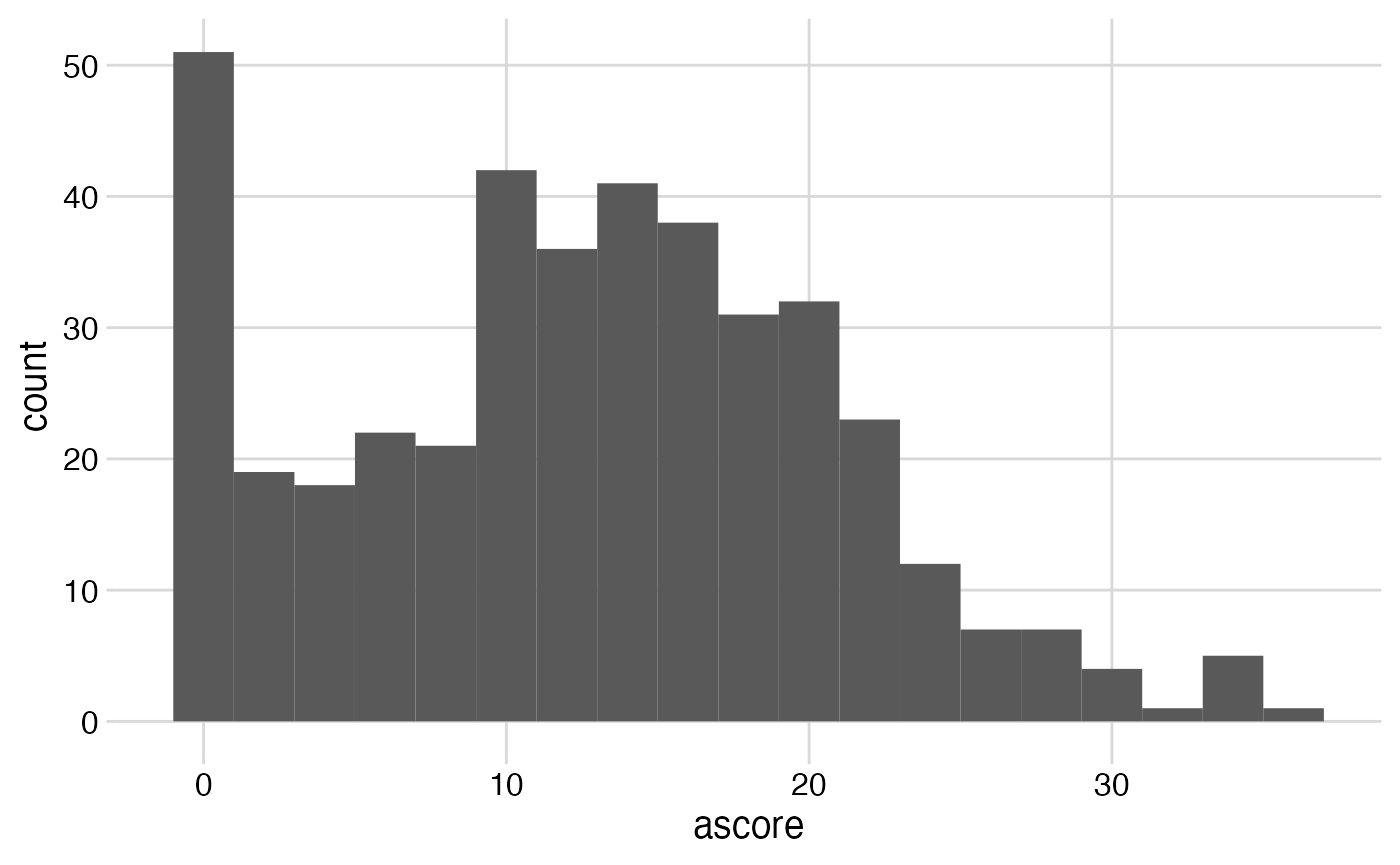
Is the outcome reasonably normally distributed? Show a quantile–quantile plot before and after log transformation.
combined %>%
  ggplot(aes(sample = ascore)) +
  stat_qq() +
  stat_qq_line() +
  labs(y = "Sample, untransformed") +
  theme_minimal_grid()
combined %>%
  ggplot(aes(sample = log(ascore + 0.1))) +
  stat_qq() +
  stat_qq_line() +
  labs(y = "Sample, log(x + 0.1)-transformed") +
  theme_minimal_grid()
Main results
Study population: Applying and documenting exclusions
Because the main exposure is self-reported race, we will have to exclude participants with missing race from the analytical population.
# All participants:
nrow(combined)
#> [1] 411

# Exclude with missing race:
analytical <- combined %>%
  filter(!is.na(race)) %>%
  copy_labels_from(from = combined)

# Analytical population:
nrow(analytical)
#> [1] 411
Note that the dataset contains participants with tumors that were metastatic at diagnosis (M1):
analytical %>%
  count(mstage)
#> # A tibble: 4 × 2
#>   mstage     n
#>   <fct>  <int>
#> 1 NULL       3
#> 2 M0       195
#> 3 M1        11
#> 4 MX       202
In the analytical dataset, does everyone have an aneuploidy score?
analytical %>%
  mutate(missing_ascore = is.na(ascore)) %>%
  tabulate_rowcol(missing_ascore, race) %>%
mygt()| missing_ascore X race | White | Asian | Black | Null | Total |
|---|---|---|---|---|---|
| FALSE | 326 | 44 | 23 | 18 | 411 |
| Total | 326 | 44 | 23 | 18 | 411 |
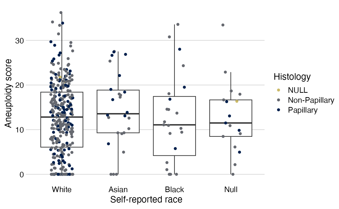
Figure 1: Box-whiskers/dot plots
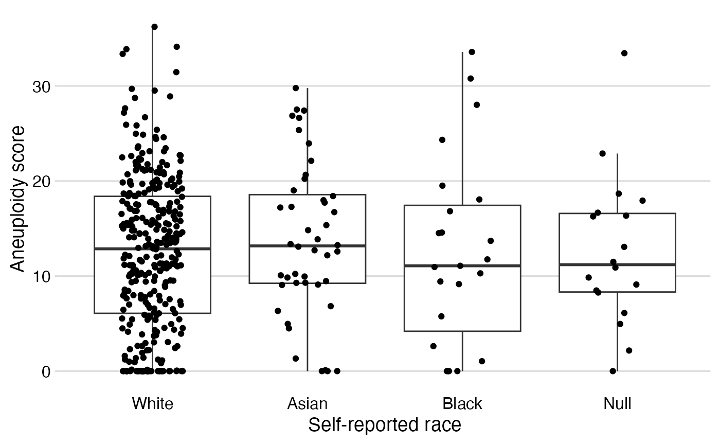
Restricted to high grade, non-missing aneuploidy scores and histology, and then color code by histology
analytical %>%
  filter(grade == "High Grade") %>%
  filter(!is.na(ascore) & !is.na(histology)) %>%
  stripplot(x = race,
            y = ascore,
            color = histology) +
  # change color palette:
  scale_color_viridis_d(option = "cividis",
                        end = 0.8,
                        direction = -1) +
  # add label:
  labs(color = "Histology")